Veri Analizi Temelleri

MBG4181 Biyolojik Veri Analizi ve Görüntüleme - Ders1

Alper Yılmaz

2026-09-28

Data Science / Veri Bilimi


Where does the time go?
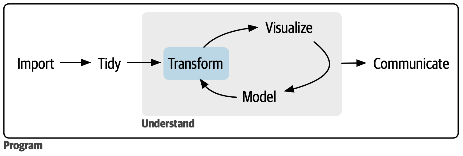


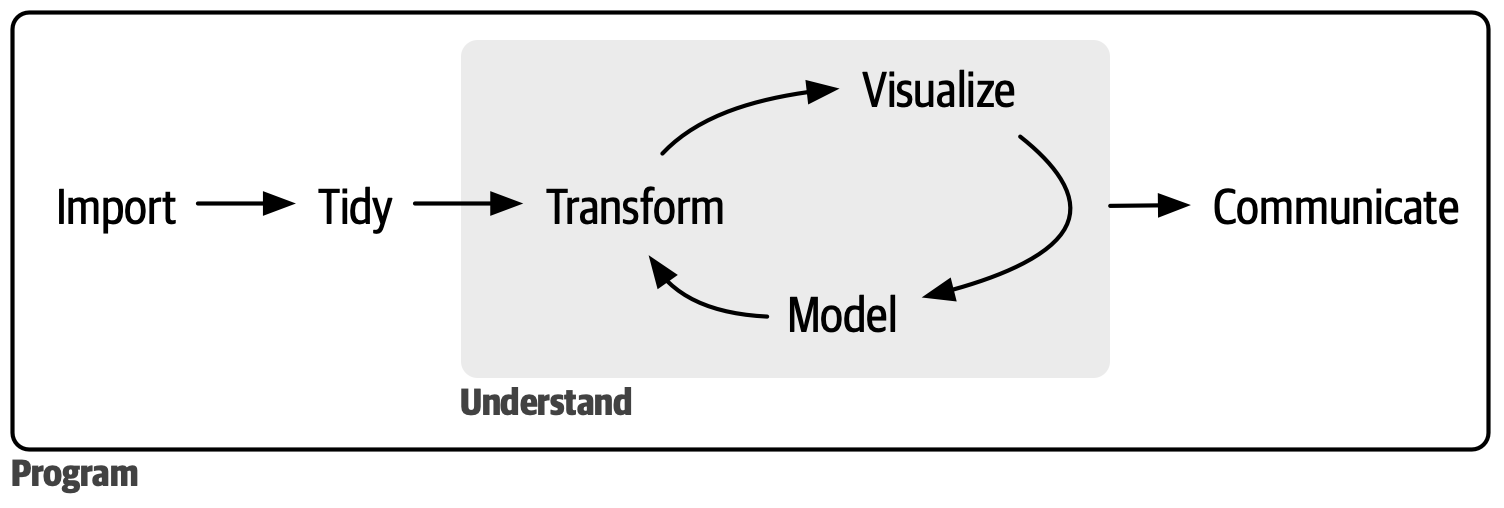
Surveys put ~80% of analysis time into getting the data ready: importing, tidying and transforming.

tidyverse makes you efficient in exactly that 80%.

Why R? / Neden R?

Tool Shines at But
Linux terminal (grep, awk, sed) quick jobs on huge text files no statistics or graphics, hard to reuse
Excel small tables, quick charts, sharing silent errors — turns gene symbols into dates (~1 in 5 papers!), not reproducible
Python (pandas + Jupyter) general purpose scripting, machine learning thinner tooling for genomics and statistics
SQL (duckdb, databases) the lingua franca of data analysis: query databases and even CSV files directly (DuckDB), scales beyond memory no statistics or graphics — pair it with R
R (tidyverse + RStudio) statistics, visualization, Bioconductor with 2,000+ biology packages base-R quirks — which we avoid with tidyverse

All five can analyze data. We’ll see SQL again in this course; for biology we pick R: Bioconductor, reproducible scripts, free.

Same analysis, four languages

Per condition: how many genes, how many with expression above 350, and what fraction?

read_csv("expr.csv") |>
  group_by(condition) |>
  summarise(n         = n(),
            n_high    = sum(expr > 350),
            frac_high = mean(expr > 350))

Reads like the question — no dialect, no hidden steps.

import pandas as pd

df = pd.read_csv("expr.csv")
df.groupby("condition").agg(
    n         = ("gene", "size"),
    n_high    = ("expr", lambda s: (s > 350).sum()),
    frac_high = ("expr", lambda s: (s > 350).mean()),
)

Same idea, but the two lambdas hide inside agg.

SELECT condition,
       COUNT(*) AS n,
       SUM(CASE WHEN expr > 350 THEN 1 ELSE 0 END)   AS n_high,
       AVG(CASE WHEN expr > 350 THEN 1.0 ELSE 0 END) AS frac_high
FROM expr
GROUP BY condition;

CASE WHEN boilerplate, twice.

awk -F, 'NR>1{n[$2]++; if($3>350) h[$2]++}
END{for(g in n) printf "%s %d %d %.2f\n", g, n[g], h[g], h[g]/n[g]}' expr.csv

$2/$3 column indexes and manual accumulators.

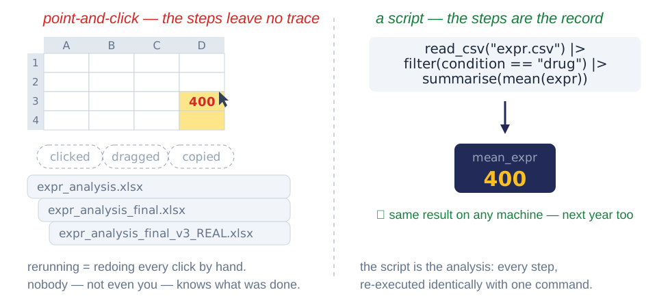
All four give the same answer — the difference is what you can still read tomorrow.

What is reproducibility?

How to run R


On your own computer

  1. Install R: cran.r-project.org
  2. Install RStudio Desktop: posit.co/download/rstudio-desktop

Free, fast, works offline.

In the cloud

Posit Cloud — a full RStudio session in your browser, nothing to install. Free student plan.


Or use nothing at all: these slides run R themselves →

R, running inside these slides

These slides carry their own R engine: webR — R compiled to WebAssembly, running in your browser. No installation, no cloud account.

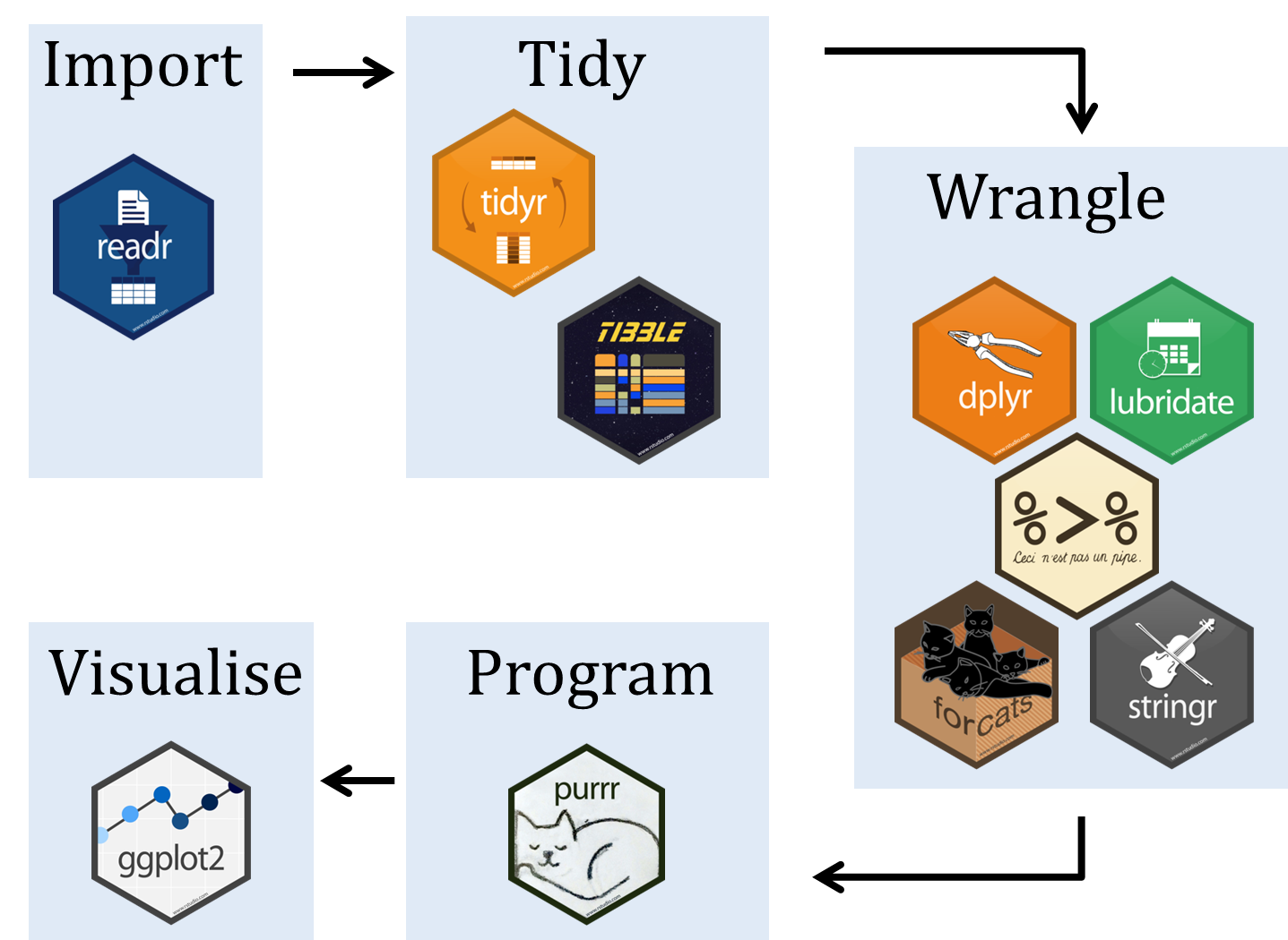
Tidyverse paketleri

Cleaning the data
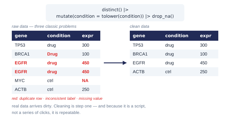
What is tidy?
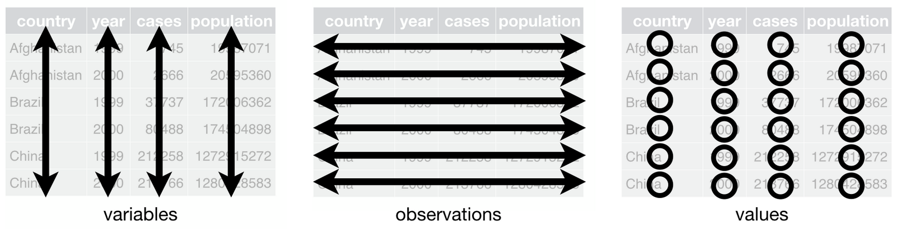

  • Variables are the columns — everything you measured: gene, condition, expr
  • Observations are the rows — one row per unit: one sample
  • Values are the cells — a single value at each variable × observation crossing

Untidy examples
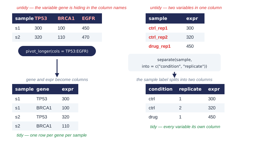
Pillars of data analysis
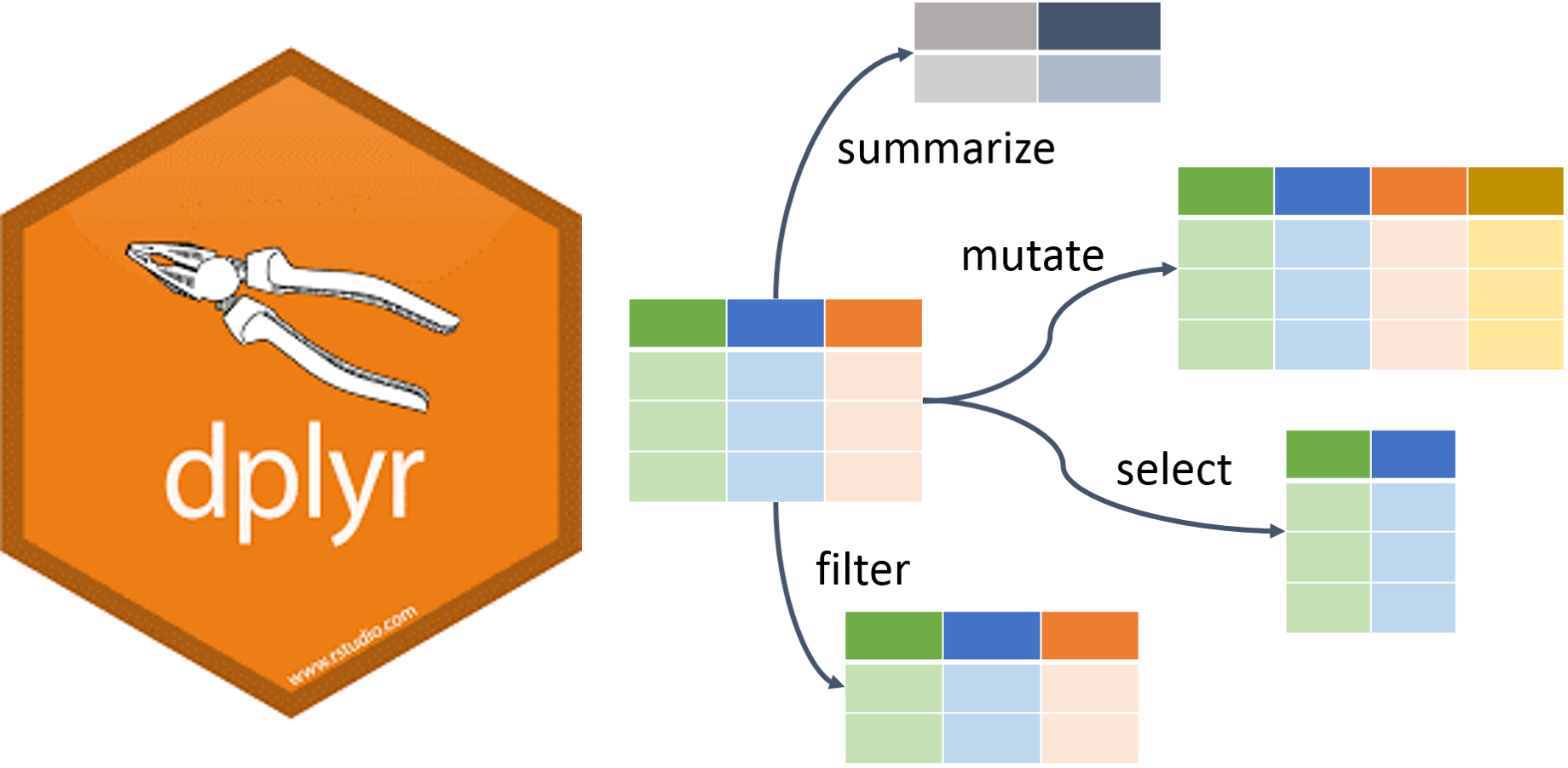
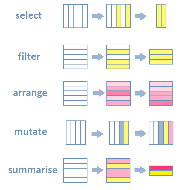
Common dplyr verbs

verb action example
filter() Select rows based on some criteria filter(age > 40 & treatment == "drug")
arrange() Sort rows arrange(date, group)
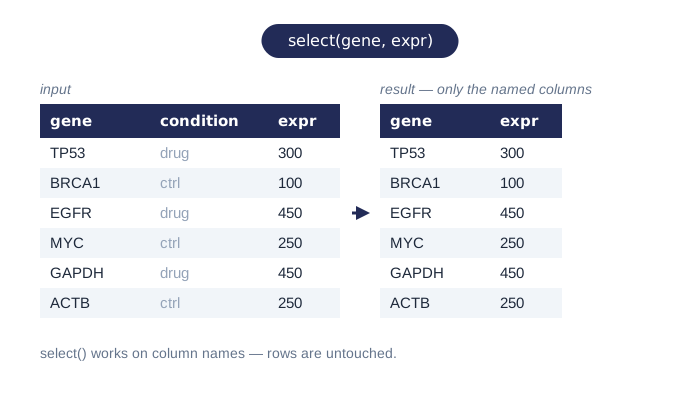
select() Select columns (and ignore all others) select(age, treatment)
rename() Rename columns rename(date = DATE_MONTHS_trial24)
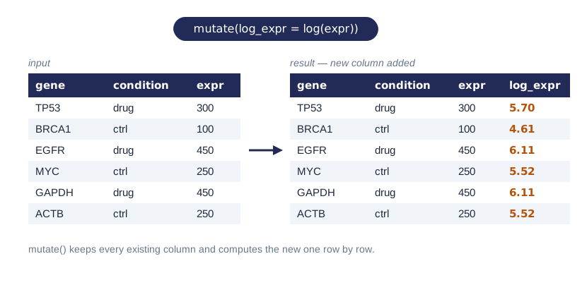
mutate() Add new columns mutate(height.m = height.cm / 100)
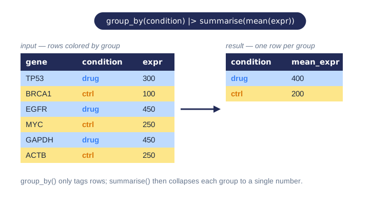
group_by(), summarise() Group data and then calculate summary statistics group_by(treatment) |> summarise(...)

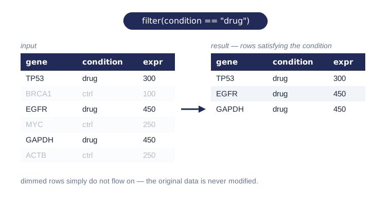
filter(): keep matching rows

select(): keep columns
mutate(): compute new columns
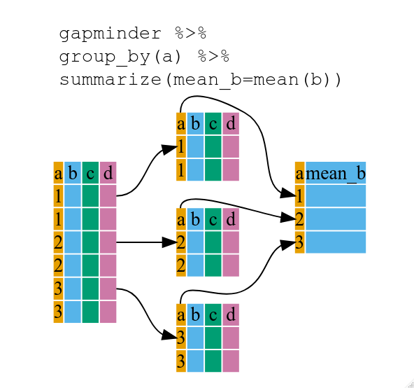
group_by() + summarise(): collapse groups
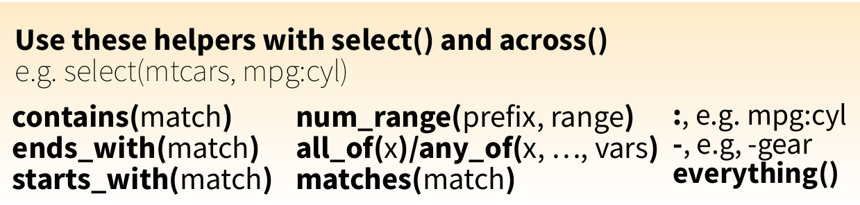
Helper functions

select might look simple but it becomes very useful with helper functions
Group by
Connecting verbs/actions - the pipe
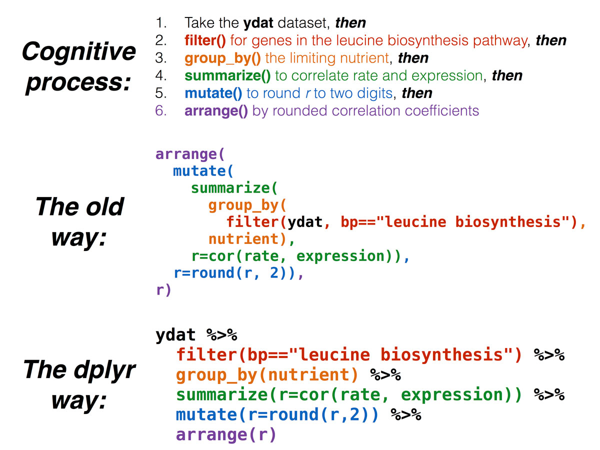

In other words

white_and_yolk <- crack(egg, add_seasoning)
omelette_batter <- beat(white_and_yolk)
omelette_with_chives <- cook(omelette_batter,add_chives)

versus

egg |>
  crack(add_seasoning) |>
  beat() |>
  cook(add_chives) -> omelette_with_chives

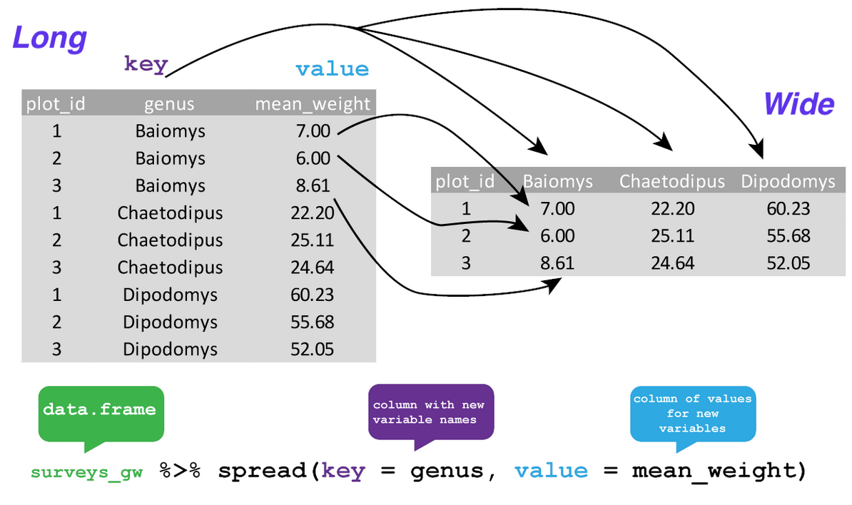
Reshaping data

Scenario 1

Scenario 2

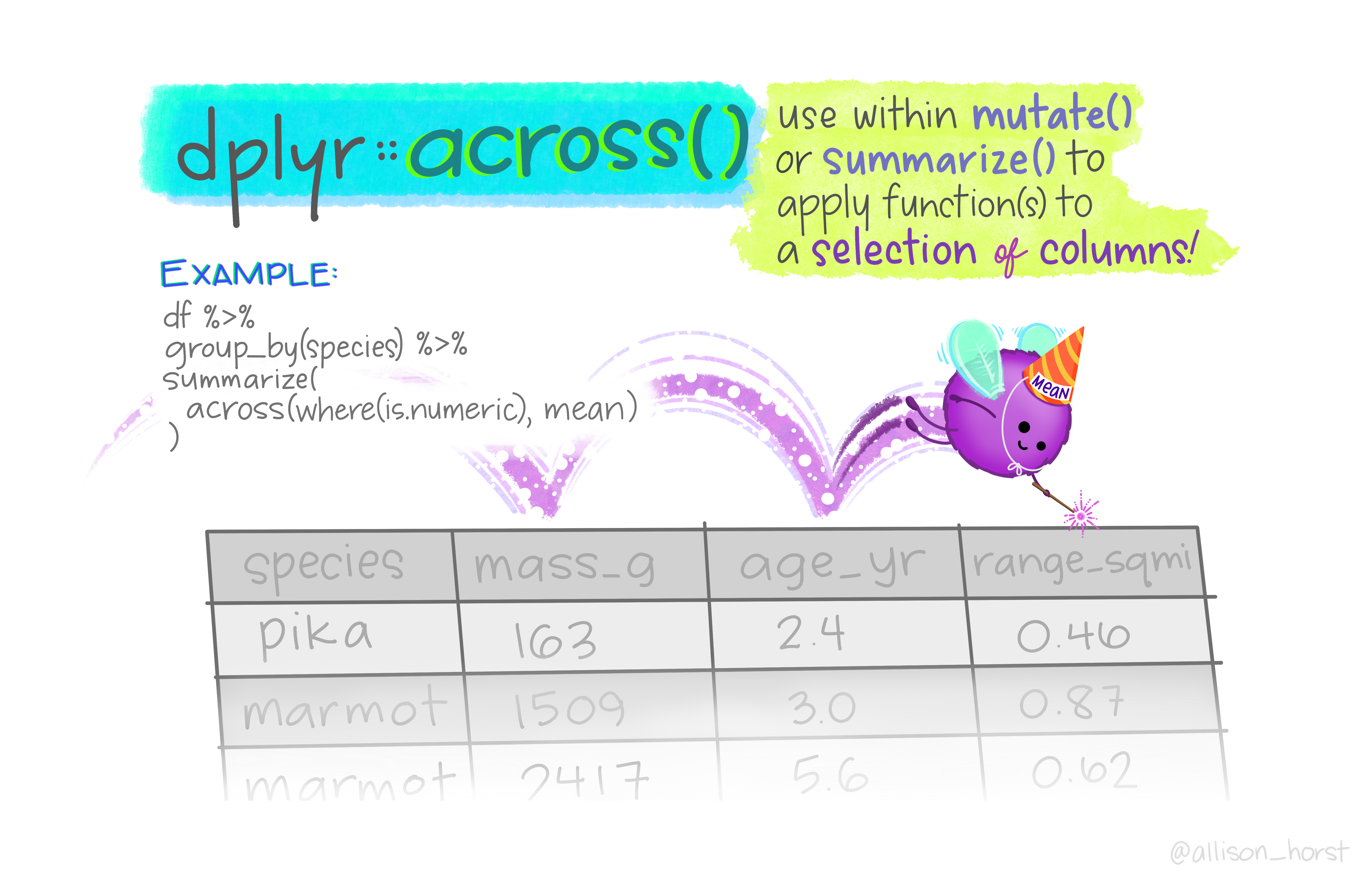
Working on multiple columns


df |>
  group_by(g1, g2) |>
  summarise(a = mean(a), b = mean(b), c = mean(c), d = mean(d))

versus

df |>
  group_by(g1, g2) |>
  summarise(across(a:d, mean))

# or with a function
df |>
  group_by(g1, g2) |>
  summarise(across(where(is.numeric), mean))

Scenario 3

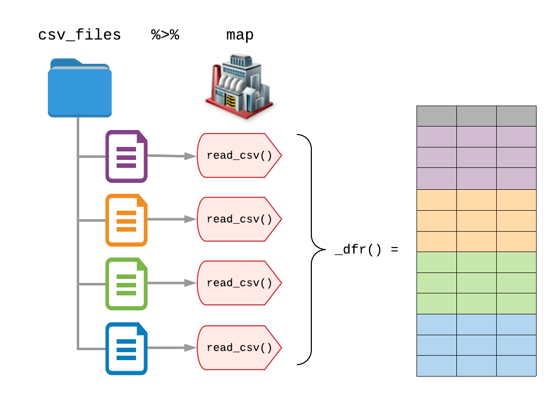
Read many files at once

fs::dir_ls(data_dir,
           regexp = "\\.csv$") |>
  map_dfr(read_csv)

Scenario 4

Combine text analysis and graph/network analysis

There are lots of packages which follow the tidyverse principles which produce and work on tidy data.

This allows mixing packages/analysis from different domains

tidytext and tidygraph packages are great examples. Former allow text analysis by converting text data to tidy data (very long data frame, one word per row) and latter imports data frames to graphs and allows access to node or edge data with dplyr verbs.

janeaustenr::austen_books() |>                              #tidytext
  unnest_tokens(bigram, text, token = "ngrams", n=2) |>     #tidytext
  filter(!is.na(bigram)) |>                                 #dplyr
  separate(bigram, into = c("word1","word2")) |>            #tidyr
  anti_join(stop_words, by=c("word1"="word")) |>            #dplyr
  anti_join(stop_words, by=c("word2"="word")) |>            #dplyr
  count(word1, word2, sort=T) |>                            #dplyr
  filter(n>20) |>                                           #dplyr
  as_tbl_graph() |>                                         #tidygraph
  mutate(central=centrality_degree(mode = "all")) |>        #dplyr/tidygraph
  ggraph(layout = 'nicely') +                                #ggraph
  geom_edge_link() +
  geom_node_point(aes(color=central)) +
  geom_node_label(aes(label=name), repel=T) +
  theme_graph()

Visualization


The popular ggplot2 package is part of tidyverse.

For stunning figures in your publications, reports you’re encouraged to use ggplot2 package

Biyoloji ve tidyverse

Bioconductor paketleri listesinde “tidy” kelimesini aratınız.