Random Forest Regression with R

# Load required libraries
library(randomForest)

randomForest 4.7-1.1

Type rfNews() to see new features/changes/bug fixes.

library(ggplot2)

Attaching package: 'ggplot2'

The following object is masked from 'package:randomForest':

    margin

# Set seed for reproducibility
set.seed(123)

data <- mtcars

Split data into training and testing sets

train_indices <- sample(1:nrow(data), 0.7 * nrow(data))
train_data <- data[train_indices, ]
test_data <- data[-train_indices, ]

Train Random Forest model and make predictions

rf_model <- randomForest(mpg ~ ., data = train_data, ntree = 500)

predictions <- predict(rf_model, newdata = test_data)

Calculate RMSE

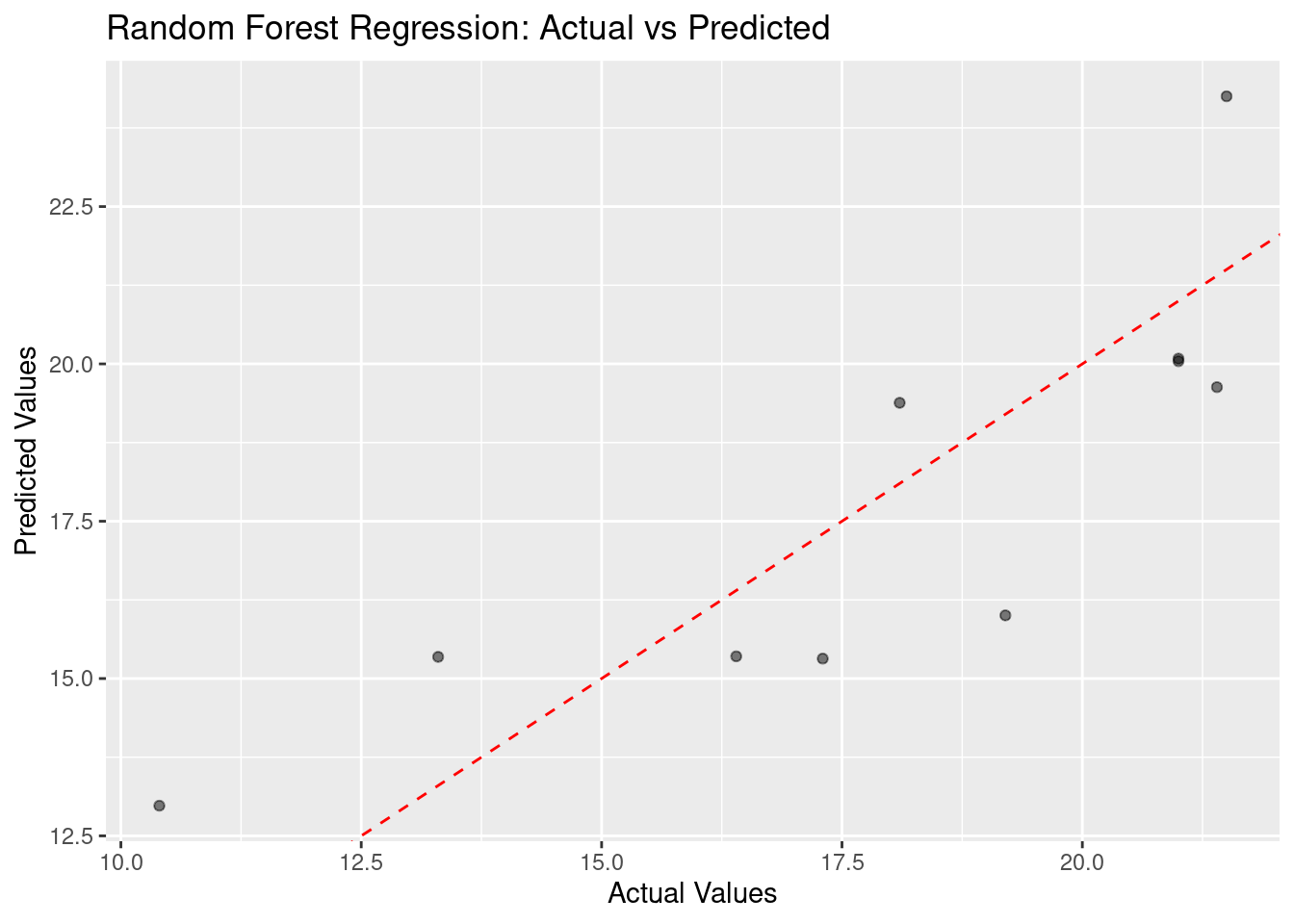
rmse <- sqrt(mean((test_data$mpg - predictions)^2))
cat("Root Mean Square Error:", rmse, "\n")

Root Mean Square Error: 2.00452 

Plot actual vs predicted values

ggplot(data.frame(actual = test_data$mpg, predicted = predictions), aes(x = actual, y = predicted)) +
  geom_point(alpha = 0.5) +
  geom_abline(intercept = 0, slope = 1, color = "red", linetype = "dashed") +
  labs(x = "Actual Values", y = "Predicted Values", title = "Random Forest Regression: Actual vs Predicted")

Print feature importance

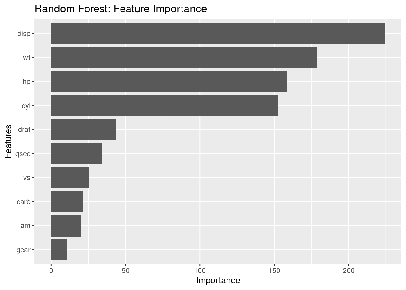
importance <- importance(rf_model)
print(importance)

     IncNodePurity
cyl      152.64821
disp     224.33387
hp       158.42647
drat      43.37372
wt       178.44424
qsec      34.05620
vs        25.67666
am        19.73485
gear      10.54314
carb      21.62506

Plot feature importance

importance_df <- data.frame(feature = rownames(importance), importance = importance[, 1])
ggplot(importance_df, aes(x = reorder(feature, importance), y = importance)) +
  geom_bar(stat = "identity") +
  coord_flip() +
  labs(x = "Features", y = "Importance", title = "Random Forest: Feature Importance")

alternative at https://hackernoon.com/random-forest-regression-in-r-code-and-interpretation