Linear Regression with R

A Polynomial Model

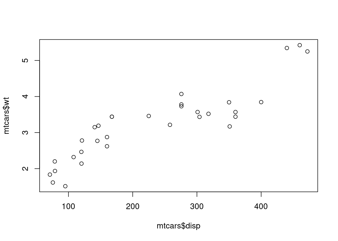
Here we have a data mtcars {datasets} that was extracted from the 1974 Motor Trend US magazine, and comprises fuel consumption and 10 aspects of automobile design and performance for 32 automobiles (1973-74 models). We will find a mathematical model between Weight (wt) and Displacement (disp) parameters. So let’s find the most suitable model. Please draw the plot, determine the degree of equation (first, second of third) and draw the curve.

mtcars

                   mpg cyl  disp  hp drat    wt  qsec vs am gear carb
Mazda RX4         21.0   6 160.0 110 3.90 2.620 16.46  0  1    4    4
Mazda RX4 Wag     21.0   6 160.0 110 3.90 2.875 17.02  0  1    4    4
Datsun 710        22.8   4 108.0  93 3.85 2.320 18.61  1  1    4    1
Hornet 4 Drive    21.4   6 258.0 110 3.08 3.215 19.44  1  0    3    1
Hornet Sportabout 18.7   8 360.0 175 3.15 3.440 17.02  0  0    3    2
Valiant           18.1   6 225.0 105 2.76 3.460 20.22  1  0    3    1
Duster 360        14.3   8 360.0 245 3.21 3.570 15.84  0  0    3    4
Merc 240D         24.4   4 146.7  62 3.69 3.190 20.00  1  0    4    2
Merc 230          22.8   4 140.8  95 3.92 3.150 22.90  1  0    4    2
 [ reached 'max' / getOption("max.print") -- omitted 23 rows ]

plot(mtcars)

plot(mtcars$disp, mtcars$wt)

first_wd <- lm(wt ~ disp, data=mtcars)
summary(first_wd)


Call:
lm(formula = wt ~ disp, data = mtcars)

Residuals:
     Min       1Q   Median       3Q      Max 
-0.89044 -0.29775 -0.00684  0.33428  0.66525 

Coefficients:
             Estimate Std. Error t value Pr(>|t|)    
(Intercept) 1.5998146  0.1729964   9.248 2.74e-10 ***
disp        0.0070103  0.0006629  10.576 1.22e-11 ***
---
Signif. codes:  0 '***' 0.001 '**' 0.01 '*' 0.05 '.' 0.1 ' ' 1

Residual standard error: 0.4574 on 30 degrees of freedom
Multiple R-squared:  0.7885,    Adjusted R-squared:  0.7815 
F-statistic: 111.8 on 1 and 30 DF,  p-value: 1.222e-11

second_wd <- lm(wt ~ disp + I(disp^2), data=mtcars)
summary(second_wd)


Call:
lm(formula = wt ~ disp + I(disp^2), data = mtcars)

Residuals:
     Min       1Q   Median       3Q      Max 
-0.88654 -0.29136 -0.00961  0.32389  0.67010 

Coefficients:
             Estimate Std. Error t value Pr(>|t|)    
(Intercept) 1.631e+00  3.622e-01   4.502 0.000101 ***
disp        6.694e-03  3.325e-03   2.013 0.053448 .  
I(disp^2)   6.206e-07  6.380e-06   0.097 0.923178    
---
Signif. codes:  0 '***' 0.001 '**' 0.01 '*' 0.05 '.' 0.1 ' ' 1

Residual standard error: 0.4652 on 29 degrees of freedom
Multiple R-squared:  0.7886,    Adjusted R-squared:  0.774 
F-statistic: 54.08 on 2 and 29 DF,  p-value: 1.639e-10

third_wd <- lm(wt ~ disp + I(disp^2) + I(disp^3), data = mtcars)
summary(third_wd)


Call:
lm(formula = wt ~ disp + I(disp^2) + I(disp^3), data = mtcars)

Residuals:
     Min       1Q   Median       3Q      Max 
-0.63764 -0.22785  0.00307  0.24614  0.58333 

Coefficients:
              Estimate Std. Error t value Pr(>|t|)    
(Intercept) -1.111e+00  5.651e-01  -1.966   0.0593 .  
disp         4.945e-02  8.198e-03   6.032 1.68e-06 ***
I(disp^2)   -1.807e-04  3.361e-05  -5.378 9.88e-06 ***
I(disp^3)    2.243e-07  4.119e-08   5.446 8.21e-06 ***
---
Signif. codes:  0 '***' 0.001 '**' 0.01 '*' 0.05 '.' 0.1 ' ' 1

Residual standard error: 0.3299 on 28 degrees of freedom
Multiple R-squared:  0.8973,    Adjusted R-squared:  0.8863 
F-statistic: 81.57 on 3 and 28 DF,  p-value: 5.959e-14

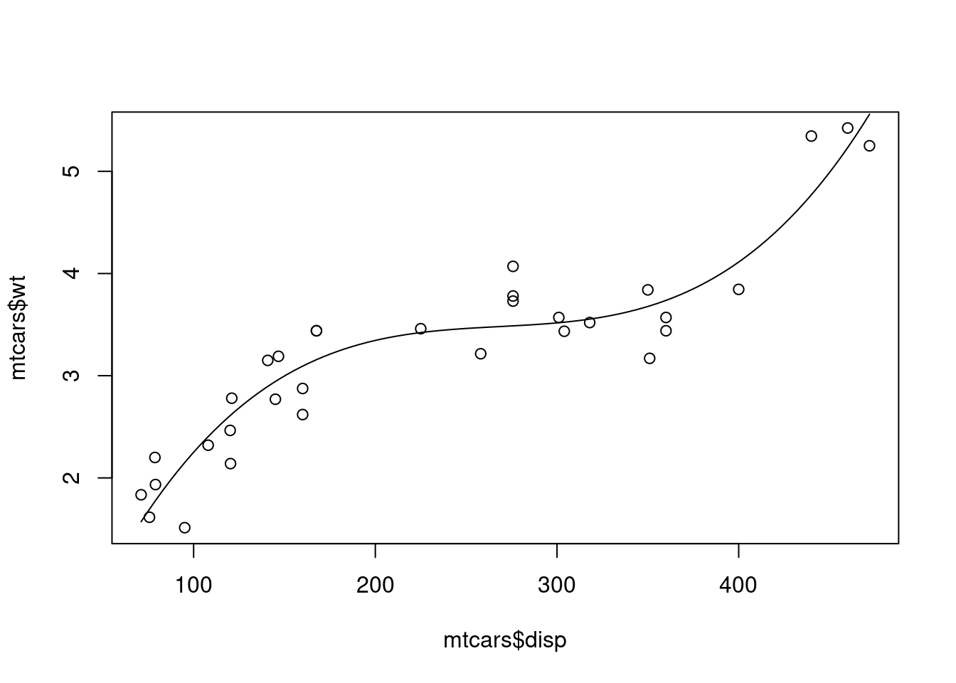
plot(mtcars$disp,mtcars$wt)
curve(2.243e-07*x^3 -1.807e-04*x^2 +4.945e-02*x -1.111e+00,add=TRUE)

best_model <- lm(wt ~ poly(disp,15), data=mtcars)
summary(best_model)


Call:
lm(formula = wt ~ poly(disp, 15), data = mtcars)

Residuals:
     Min       1Q   Median       3Q      Max 
-0.43800 -0.11202 -0.00364  0.16319  0.37783 

Coefficients:
                   Estimate Std. Error t value Pr(>|t|)    
(Intercept)       3.2172500  0.0509709  63.119  < 2e-16 ***
poly(disp, 15)1   4.8375552  0.2883350  16.778 1.41e-11 ***
poly(disp, 15)2   0.0452475  0.2883350   0.157   0.8773    
poly(disp, 15)3   1.7965723  0.2883350   6.231 1.20e-05 ***
poly(disp, 15)4   0.4463962  0.2883350   1.548   0.1411    
poly(disp, 15)5  -0.6866393  0.2883350  -2.381   0.0300 *  
poly(disp, 15)6  -0.3384161  0.2883350  -1.174   0.2577    
poly(disp, 15)7  -0.6134397  0.2883350  -2.128   0.0493 *  
poly(disp, 15)8   0.0528245  0.2883350   0.183   0.8569    
poly(disp, 15)9   0.0814084  0.2883350   0.282   0.7813    
poly(disp, 15)10 -0.0654665  0.2883350  -0.227   0.8233    
poly(disp, 15)11  0.2853853  0.2883350   0.990   0.3370    
poly(disp, 15)12 -0.0007108  0.2883350  -0.002   0.9981    
poly(disp, 15)13  0.4495723  0.2883350   1.559   0.1385    
poly(disp, 15)14 -0.0699728  0.2883350  -0.243   0.8113    
poly(disp, 15)15 -0.5031480  0.2883350  -1.745   0.1002    
---
Signif. codes:  0 '***' 0.001 '**' 0.01 '*' 0.05 '.' 0.1 ' ' 1

Residual standard error: 0.2883 on 16 degrees of freedom
Multiple R-squared:  0.9552,    Adjusted R-squared:  0.9132 
F-statistic: 22.73 on 15 and 16 DF,  p-value: 5.551e-08

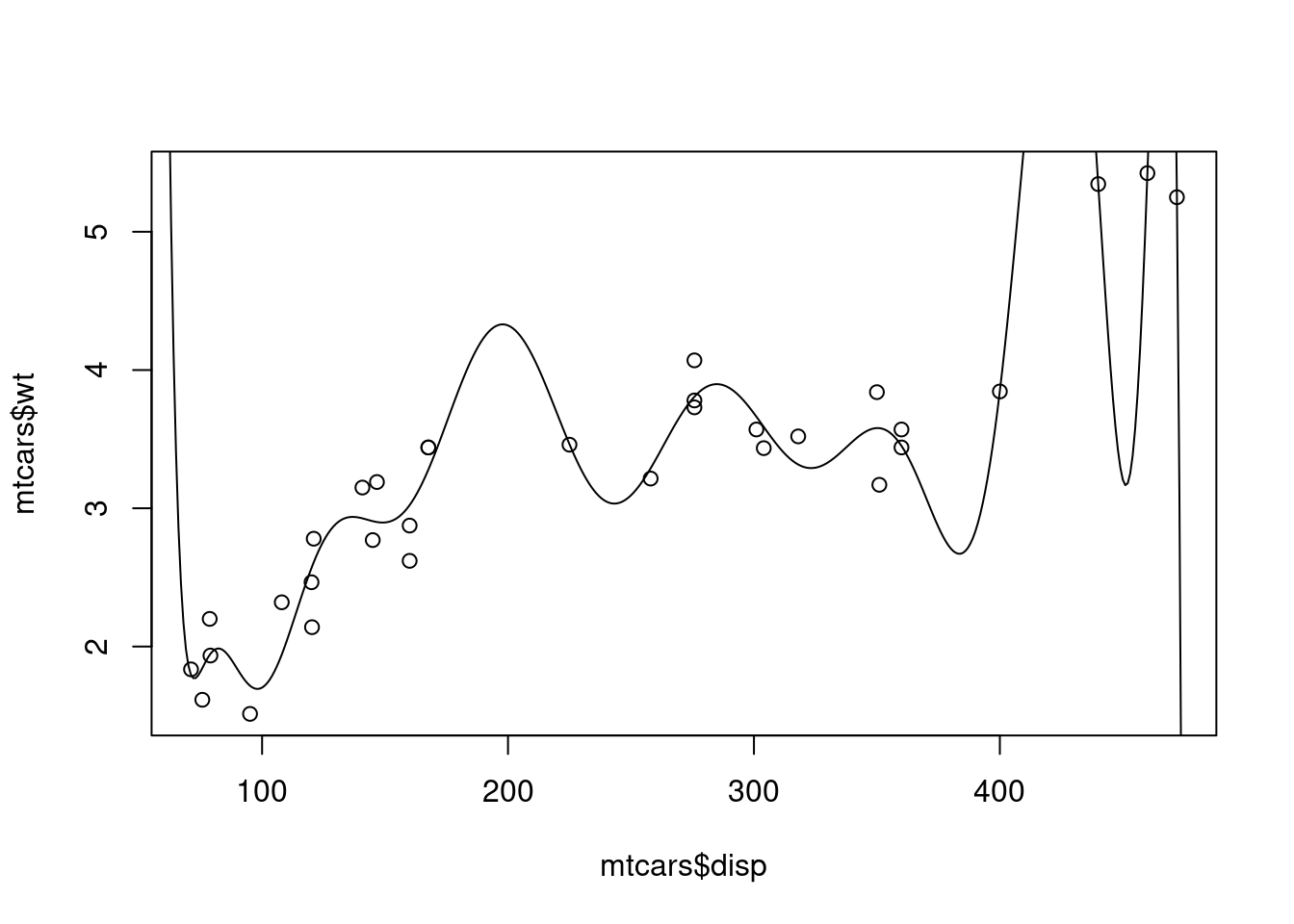
pred <- predict(best_model, data.frame(disp=50:500))
plot(mtcars$disp, mtcars$wt)
points(50:500, pred, type="l")

predict(third_wd, data.frame(disp=420))

       1 
4.397246

predict(best_model, data.frame(disp=420))

       1 
7.329183

predict(best_model, data.frame(disp=c(20,420, 500)))

           1            2            3 
 3865.329736     7.329183 -1513.538298

So, the “best” model is not best at all..

Train/Test split

Let’s understand the topic of overfitting.

Split the data into train and test. Train the model with “training” data. Then predict with “test” data.

sample(1:32, 5, replace=FALSE)

[1]  1 11 22 13 30

set.seed(2)
idx <- sample(1:32, 5, replace=FALSE)
idx

[1] 21 15  6 30  8

test <- mtcars[idx,]

test

                    mpg cyl  disp  hp drat    wt  qsec vs am gear carb
Toyota Corona      21.5   4 120.1  97 3.70 2.465 20.01  1  0    3    1
Cadillac Fleetwood 10.4   8 472.0 205 2.93 5.250 17.98  0  0    3    4
Valiant            18.1   6 225.0 105 2.76 3.460 20.22  1  0    3    1
Ferrari Dino       19.7   6 145.0 175 3.62 2.770 15.50  0  1    5    6
Merc 240D          24.4   4 146.7  62 3.69 3.190 20.00  1  0    4    2

train <- mtcars[-idx,]
train

                   mpg cyl  disp  hp drat    wt  qsec vs am gear carb
Mazda RX4         21.0   6 160.0 110 3.90 2.620 16.46  0  1    4    4
Mazda RX4 Wag     21.0   6 160.0 110 3.90 2.875 17.02  0  1    4    4
Datsun 710        22.8   4 108.0  93 3.85 2.320 18.61  1  1    4    1
Hornet 4 Drive    21.4   6 258.0 110 3.08 3.215 19.44  1  0    3    1
Hornet Sportabout 18.7   8 360.0 175 3.15 3.440 17.02  0  0    3    2
Duster 360        14.3   8 360.0 245 3.21 3.570 15.84  0  0    3    4
Merc 230          22.8   4 140.8  95 3.92 3.150 22.90  1  0    4    2
Merc 280          19.2   6 167.6 123 3.92 3.440 18.30  1  0    4    4
Merc 280C         17.8   6 167.6 123 3.92 3.440 18.90  1  0    4    4
 [ reached 'max' / getOption("max.print") -- omitted 18 rows ]

third_deg <- lm(wt ~ poly(disp,3), data = train)
summary(third_deg)$r.squared

[1] 0.8879368

predict(third_deg, test)

     Toyota Corona Cadillac Fleetwood            Valiant       Ferrari Dino 
          2.633774           5.824101           3.418857           2.970499 
         Merc 240D 
          2.989188

test$third_pred <- predict(third_deg, test)
test

                    mpg cyl  disp  hp drat    wt  qsec vs am gear carb
Toyota Corona      21.5   4 120.1  97 3.70 2.465 20.01  1  0    3    1
Cadillac Fleetwood 10.4   8 472.0 205 2.93 5.250 17.98  0  0    3    4
Valiant            18.1   6 225.0 105 2.76 3.460 20.22  1  0    3    1
Ferrari Dino       19.7   6 145.0 175 3.62 2.770 15.50  0  1    5    6
Merc 240D          24.4   4 146.7  62 3.69 3.190 20.00  1  0    4    2
                   third_pred
Toyota Corona        2.633774
Cadillac Fleetwood   5.824101
Valiant              3.418857
Ferrari Dino         2.970499
Merc 240D            2.989188

fifteen_deg <- lm(wt ~ poly(disp,15), data=train)
summary(fifteen_deg)$r.squared

[1] 0.9550231

predict(fifteen_deg, test)

     Toyota Corona Cadillac Fleetwood            Valiant       Ferrari Dino 
          2.644378        -844.610091           2.784157           2.761685 
         Merc 240D 
          2.745391

test$fifteen <- predict(fifteen_deg, test)

test[c("disp","wt","third_pred","fifteen")]

                    disp    wt third_pred     fifteen
Toyota Corona      120.1 2.465   2.633774    2.644378
Cadillac Fleetwood 472.0 5.250   5.824101 -844.610091
Valiant            225.0 3.460   3.418857    2.784157
Ferrari Dino       145.0 2.770   2.970499    2.761685
Merc 240D          146.7 3.190   2.989188    2.745391

As you can see, “fifteenth degree” model memorized (i.e overfitted) the data and predicts horribly.