K-means clustering with R

taken from Partitional Clustering in R: The Essentials

The data

library(factoextra)
data("USArrests")
df <- scale(USArrests)

head(df)

               Murder   Assault   UrbanPop         Rape
Alabama    1.24256408 0.7828393 -0.5209066 -0.003416473
Alaska     0.50786248 1.1068225 -1.2117642  2.484202941
Arizona    0.07163341 1.4788032  0.9989801  1.042878388
Arkansas   0.23234938 0.2308680 -1.0735927 -0.184916602
California 0.27826823 1.2628144  1.7589234  2.067820292
Colorado   0.02571456 0.3988593  0.8608085  1.864967207

What should K be?

fviz_nbclust(df, kmeans, "wss")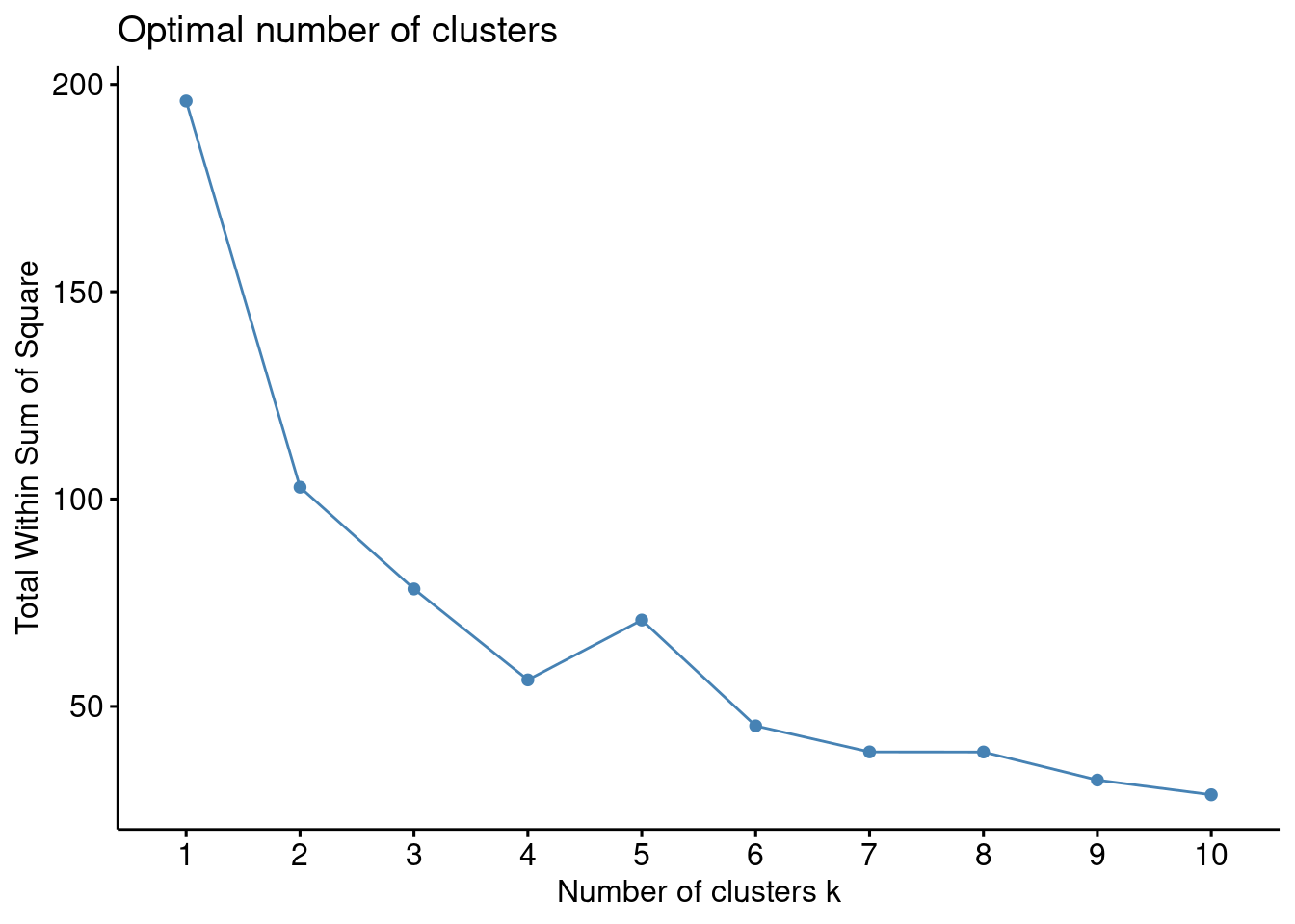

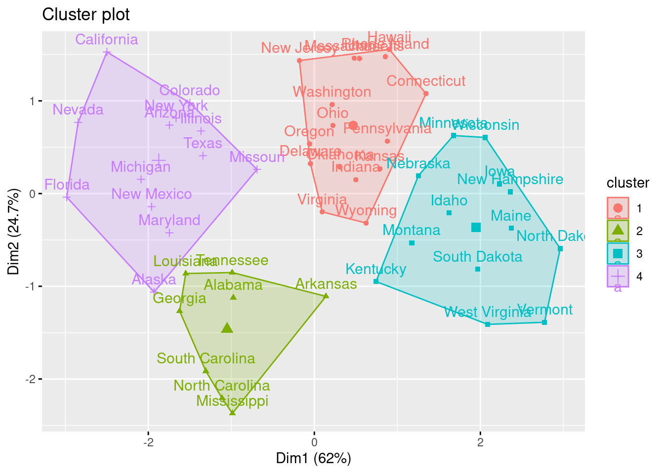
Clustering

km.res <- kmeans(df, 4, nstart=25)
print(km.res)

K-means clustering with 4 clusters of sizes 16, 8, 13, 13

Cluster means:
      Murder    Assault   UrbanPop        Rape
1 -0.4894375 -0.3826001  0.5758298 -0.26165379
2  1.4118898  0.8743346 -0.8145211  0.01927104
3 -0.9615407 -1.1066010 -0.9301069 -0.96676331
4  0.6950701  1.0394414  0.7226370  1.27693964

Clustering vector:
       Alabama         Alaska        Arizona       Arkansas     California 
             2              4              4              2              4 
      Colorado    Connecticut       Delaware        Florida        Georgia 
             4              1              1              4              2 
        Hawaii          Idaho       Illinois        Indiana           Iowa 
             1              3              4              1              3 
        Kansas       Kentucky      Louisiana          Maine       Maryland 
             1              3              2              3              4 
 Massachusetts       Michigan      Minnesota    Mississippi       Missouri 
             1              4              3              2              4 
       Montana       Nebraska         Nevada  New Hampshire     New Jersey 
             3              3              4              3              1 
    New Mexico       New York North Carolina   North Dakota           Ohio 
             4              4              2              3              1 
      Oklahoma         Oregon   Pennsylvania   Rhode Island South Carolina 
             1              1              1              1              2 
  South Dakota      Tennessee          Texas           Utah        Vermont 
             3              2              4              1              3 
      Virginia     Washington  West Virginia      Wisconsin        Wyoming 
             1              1              3              3              1 

Within cluster sum of squares by cluster:
[1] 16.212213  8.316061 11.952463 19.922437
 (between_SS / total_SS =  71.2 %)

Available components:

[1] "cluster"      "centers"      "totss"        "withinss"     "tot.withinss"
[6] "betweenss"    "size"         "iter"         "ifault"      

Visualizing the results

fviz_cluster(km.res, data=df)