Excel - Part2
FEF1002 - Lecture5
Week 5: Excel - Part2
This module will cover the following concepts:
- Sorting, Filtering, Conditional Formatting
- Writing Functions in Excel
Sorting, Filtering, Conditional Formatting
Sorting
Sorting data is an integral part of data analysis. You might want to organize a name list in alphabetical order, compile a product stock levels list from highest to lowest, or sort rows by colors or icons. Sorting data helps you better see and understand your data, find and organize the data you want, and ultimately make much more effective decisions.
Text Sorting
Select a cell in the column you want to sort.
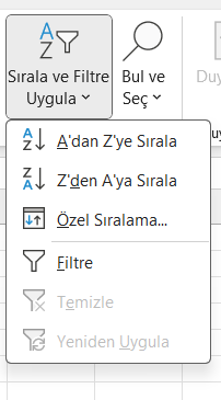
In the Data tab, in the Sort and Filter group, do one of the following:
For quick ascending order sorting, click the A to Z command (Sort A to Z) which sorts in Excel from A to Z or from smallest to largest number.
For quick descending order sorting, click the Z to A command (Sort Z to A) which sorts in Excel from Z to A or from largest to smallest number.
Number Sorting
Select a cell in the column you want to sort.
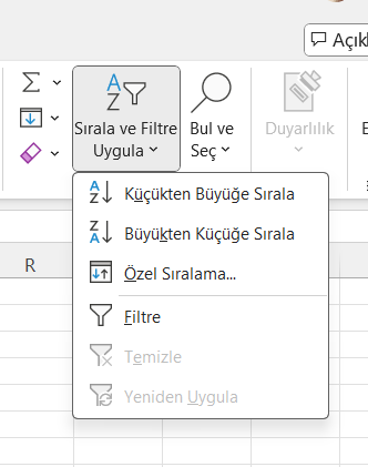
In the Data tab, in the Sort and Filter group, do one of the following:
To sort from smallest to largest, click the A to Z command (Sort Smallest to Largest) which sorts in Excel from smallest to largest number.
To sort from largest to smallest, click the Z to A command (Sort Largest to Smallest) which sorts in Excel from largest to smallest number.
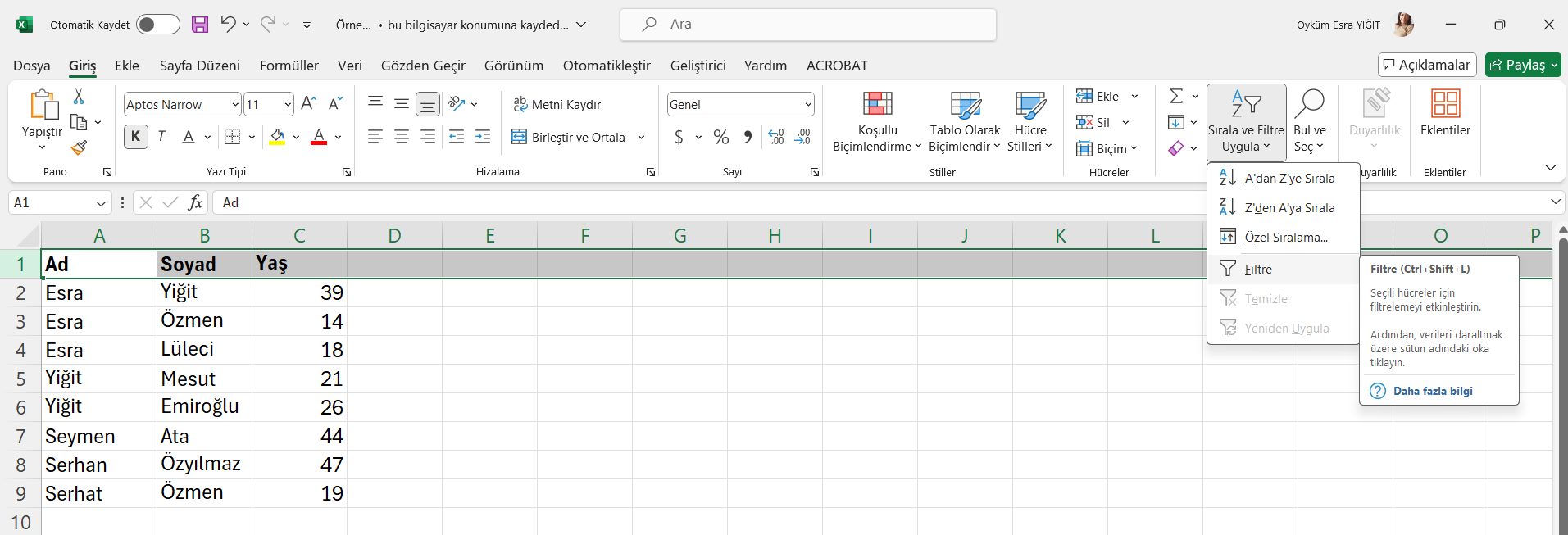
Filtering
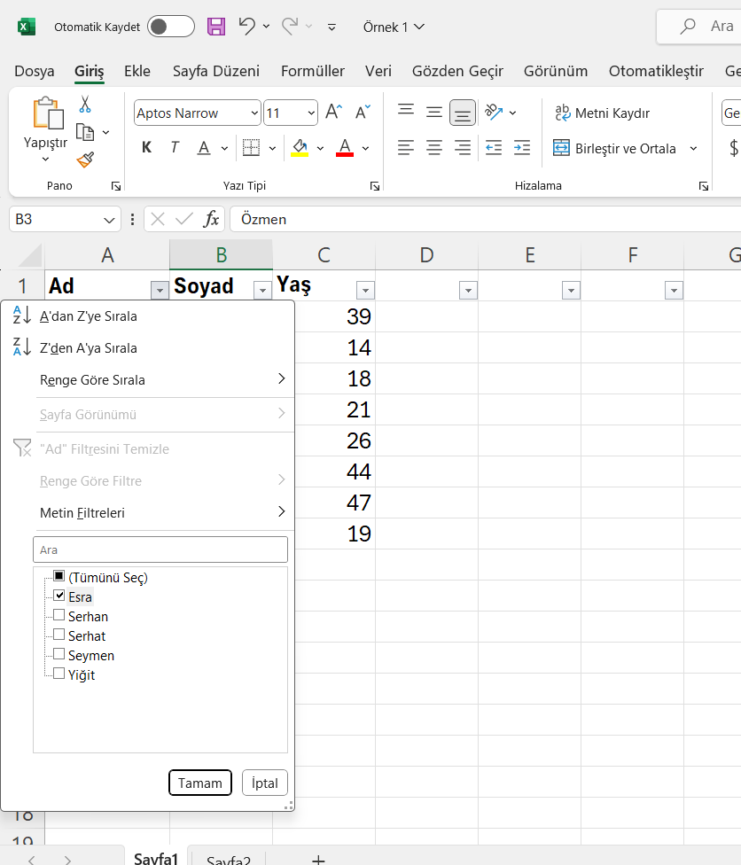
Filtering an Entire Column
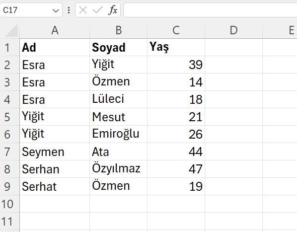
Please use the sample Excel file ornek1.xlsx for the following samples.
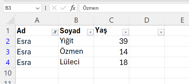
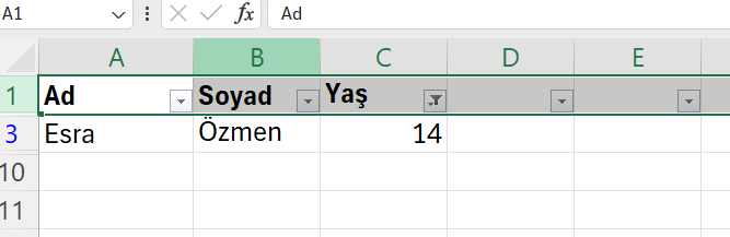
Let’s enter the following data and find all cells with the name Esra.
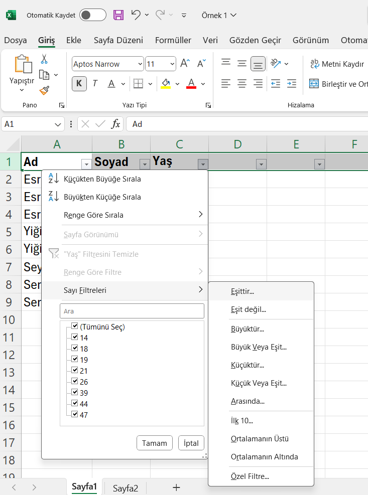
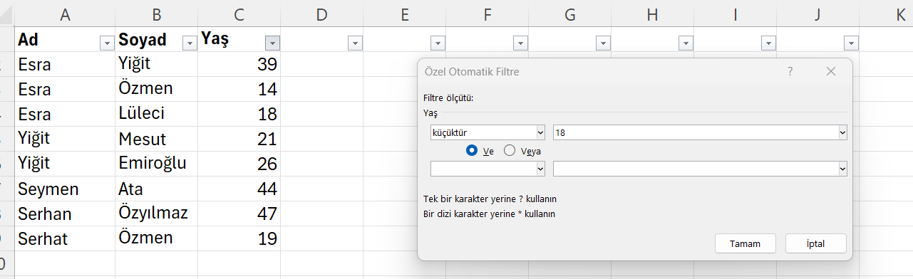
Filtering Specific Numbers
Let’s filter those younger than 18 in the same example
Conditional Formatting
Conditional formatting can help make patterns and trends in your data more apparent. It works with the logic of if… then…. If cell content has a specific value according to certain criteria, that cell’s formatting changes according to the selected option or any format you desire. You can change formatting elements such as cell background color, borders, fonts, and you can also display icons in the cell. In other words, it allows you to see values that are more important or special to you more easily at first glance. You can even use it for error checking; for example, in a formula that multiplies values from different cells for a subtotal, you can use formatting that will quickly show you cells that don’t return values.
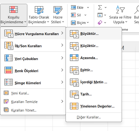
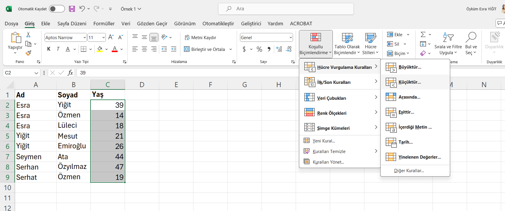
Cell Highlighting Rules
As shown below, you can select one of the preset formats in cell highlighting rules or create custom formatting.
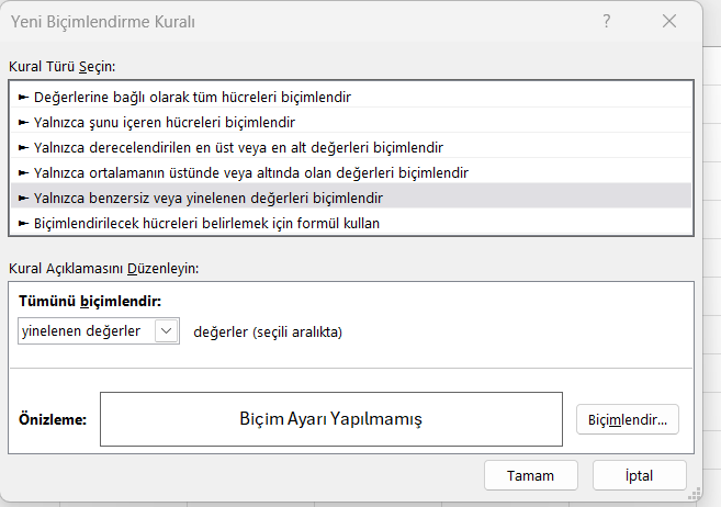
The formatting option includes “Greater Than”, “Less Than”, “Between”, “Equal To”, “Text Contains”, “Date” and “Duplicate Value”. For example, when “Duplicate” is clicked, an additional window appears with a dropdown box where you can select “Duplicate” or “Unique” options to format repeated values or unique values.
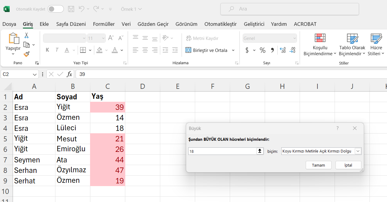
For example, let’s highlight those over 18 years old
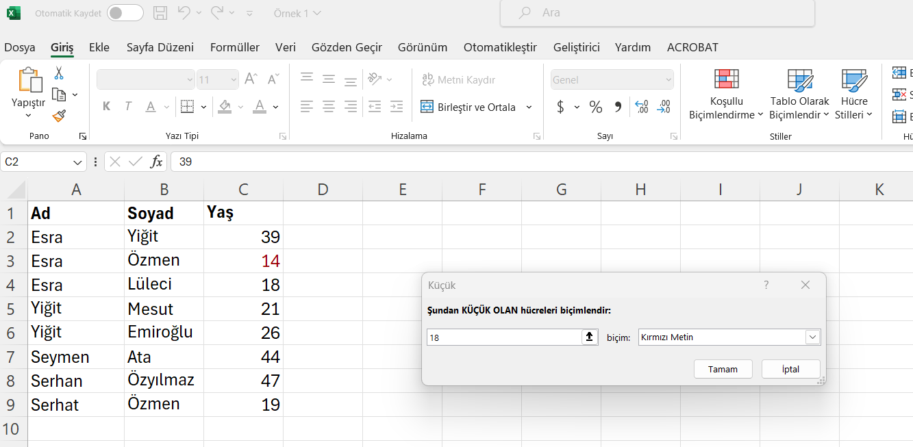
Similarly, let’s highlight those under 18 years old
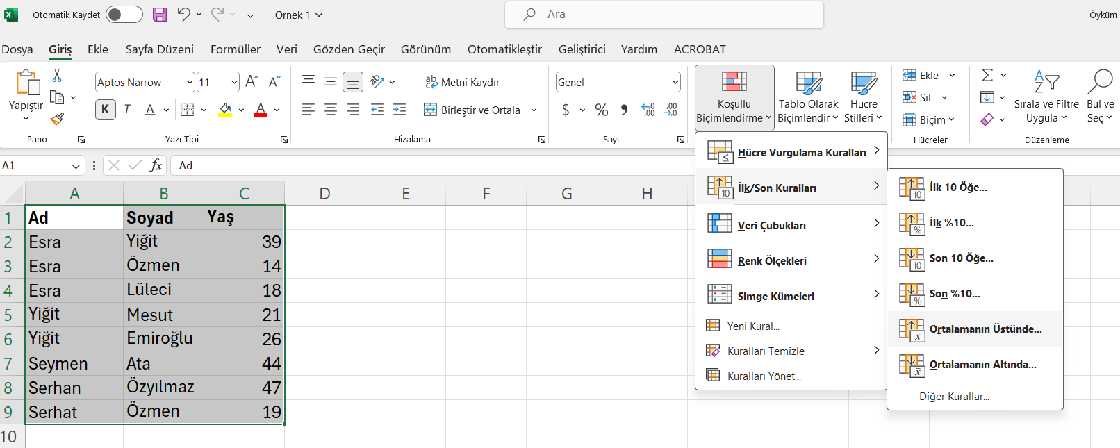
Top/Bottom Rules
With this option, you can select self-explanatory preferences including top 10, top 10%, bottom 10, bottom 10%, below average, and above average in your selected range.
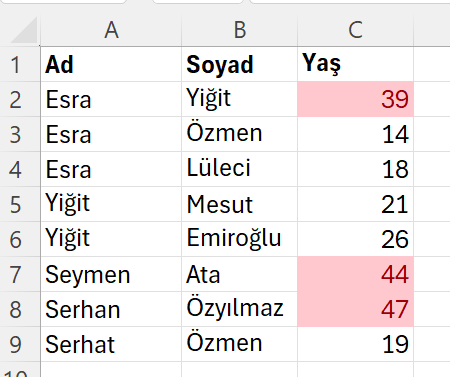
Let’s highlight the data above average
Similarly, to highlight repeated or unique values, you just need to select other rules option.
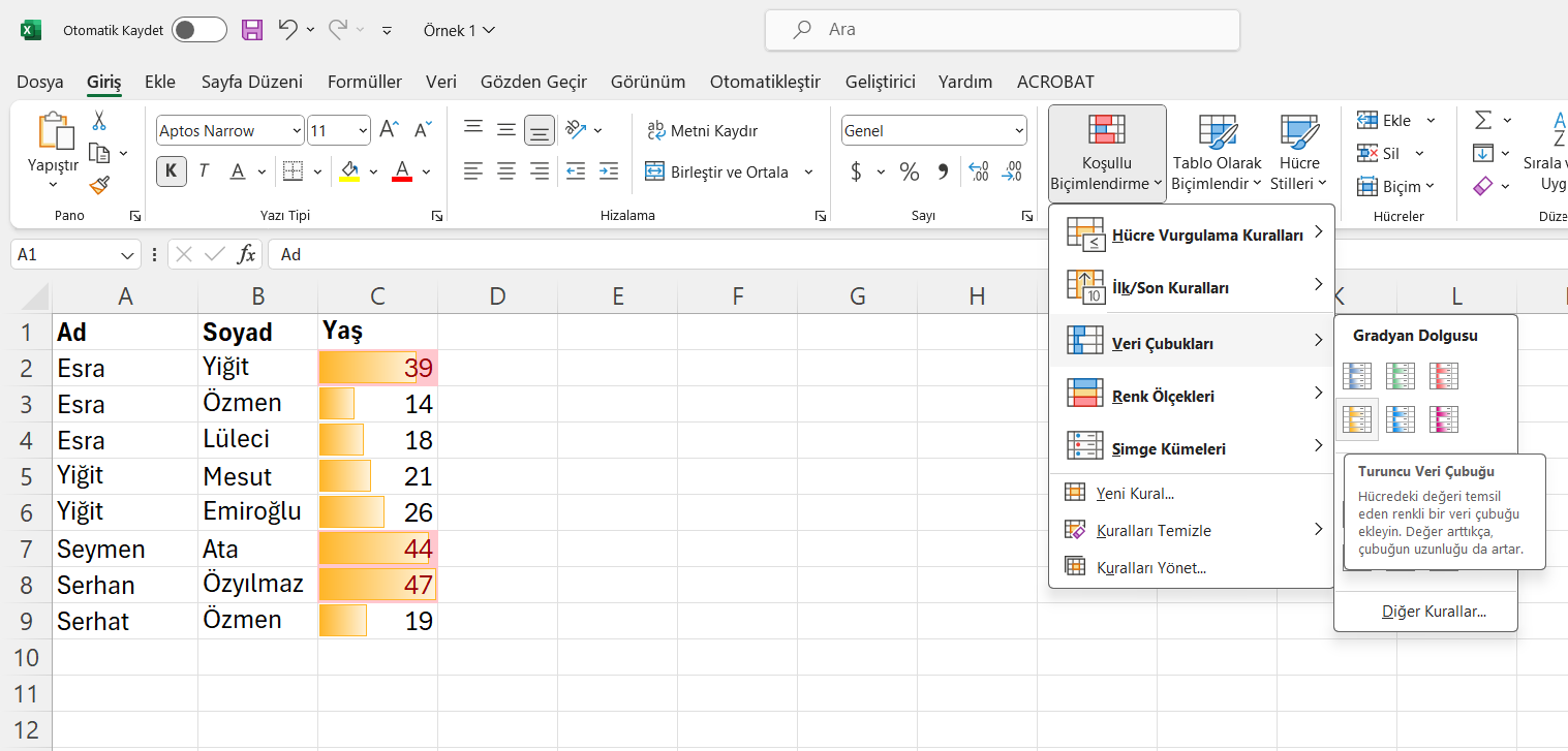
Data Bars
Data bars fill cells with horizontal bar graphs according to the values in your selected range, with the largest value filling the entire cell horizontally and other values scaled proportionally in comparison.
If you click on Other Rules, you can apply formatting according to your own preferences or formula through a form. Additionally, you can modify the fill and border of the bars within cells to create custom formatting.
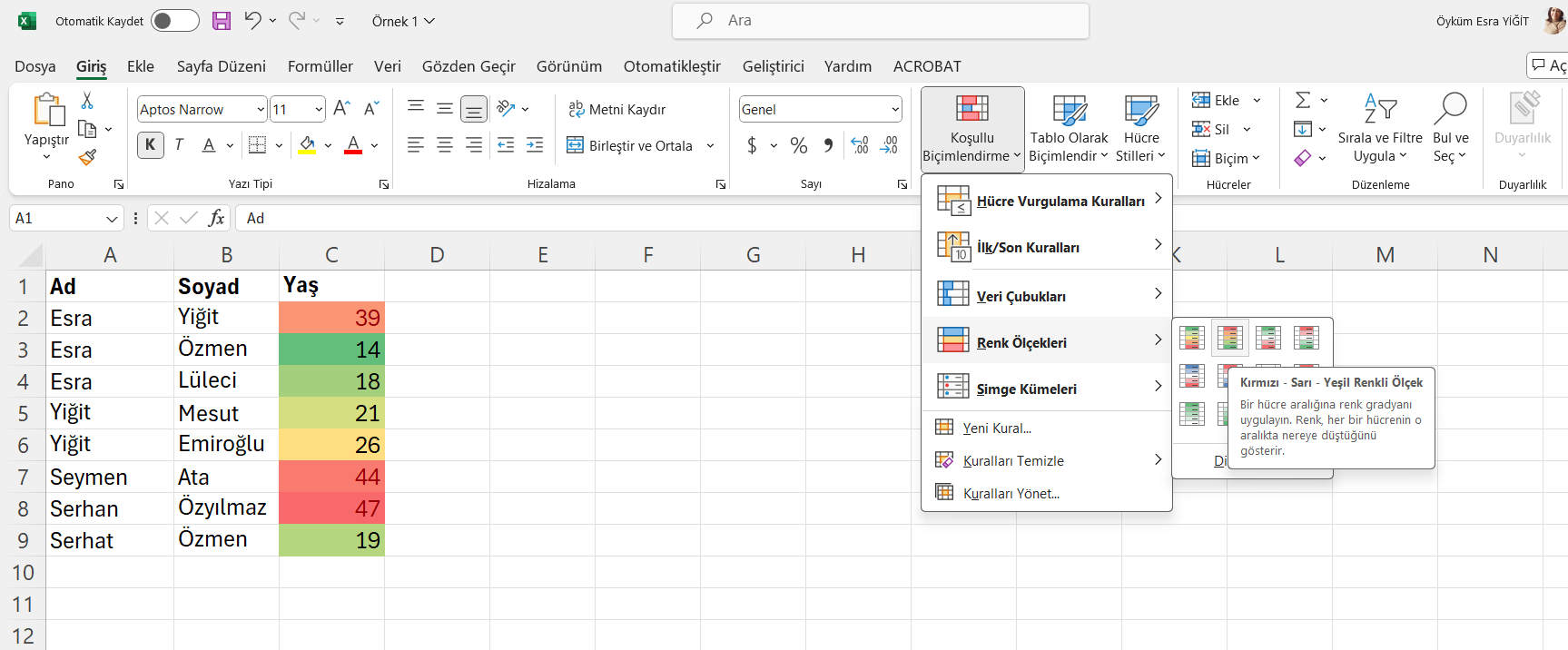
Color Scales
This option creates a scale between the largest and smallest values in your selected range and adjusts the cell fill color according to the scale between two colors you choose.
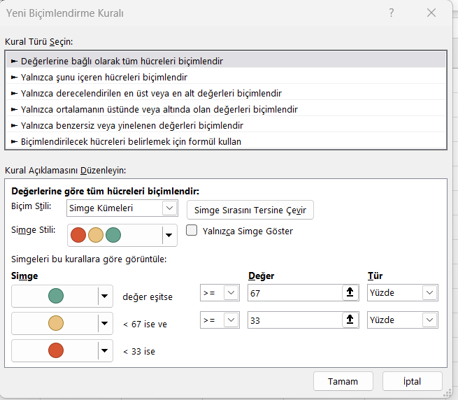
Icon Sets
Icon sets show different symbols next to the value in the cell indicating which range the value falls into based on a scale between the largest and smallest values in your selected range. You can create rules and assign icons according to your rules.
Writing Functions in EXCEL
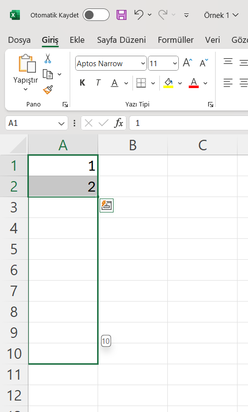
Entering Data Series
When you need to enter sequential numbers like serial numbers in a table, instead of typing these numbers one by one manually, we can enter them using the auto-fill method. For this:
- Enter the first two sequence numbers in cells either vertically or horizontally.
- Select these two cells, starting with the cell containing the first number.
- Take the mouse pointer to the fill handle (small dot) in the bottom right corner of the selected area (mouse pointer becomes a small plus), hold down the left mouse button and drag down or to the side.
Note: You determine the rule. If the first two cells contain 2 and 4, you will create numbers increasing by 2.
Formula Creation
You can perform calculations using formulas in Excel tables. When entering a formula into a cell, you need to pay attention to the following:
- Formulas start with = sign
- No spaces should be given when writing formulas (except for text in quotes within the formula)
- The number of opening parentheses should match the number of closing parentheses
- Constant numbers, cell names, and range names can be used when writing formulas
- F2 key is used to edit the formula
- DELETE key is used to delete the formula
- ESC key is used to exit the formula
- Formulas can be replicated
- Addition and multiplication operations have functions. However, division and subtraction operations don’t have functions
- Colon: Includes the cell range in the operation. For example, if A2:A8, all cells from A2 to A8 are included in the operation
- Semicolon; Only includes those specific cells in the operation. Does not take the range. For example, if A2;A8, only A2 and A8 are included in the operation
- If the value in the formula is a number, it is written directly. For example; A2=50
- If the value in the formula is a word, it is written in quotes. For example; A2=“female”
- During formula replication, cell fixing can be done to prevent cell changes. Press F4 key to fix a cell. Or it can be fixed by writing manually.

Source: HANIFE BOZKURT BATMAN
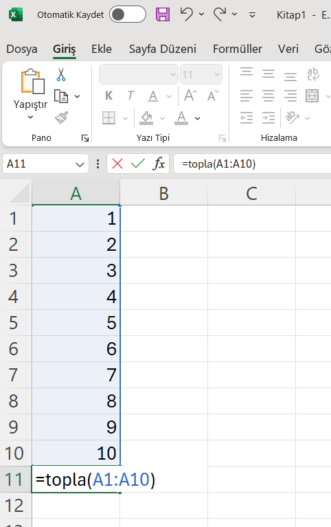
Addition Operation
=SUM(A1:A10) Performs Addition Operation. Adds Cells from A1 to A10.
Multiplication Operation
=PRODUCT(A1:A10) Performs Multiplication Operation. Multiplies Cells from A1 to A10. 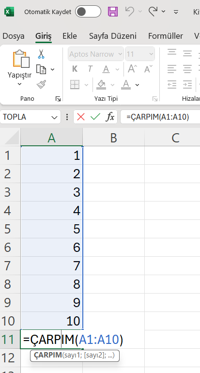
=AVERAGE(A1:A10) Calculates Average. Finds the Average of Cells from A1 to A10.
=MAX(A1:A10) Finds the Largest Number. Finds the Highest Number in Cells from A1 to A10.
=MIN(A1:A10) Finds the Smallest Number. Finds the Smallest Number in Cells from A1 to A10.
=SMALL(A1:A10;2) Returns the SMALL number in the Range. However, which small number is required must be specified in the formula. Finds the 2nd smallest number from A1 to A10.
=LARGE(A1:A10;3) Returns the LARGE number in the Range. However, which large number is required must be specified in the formula. Finds the 3rd largest number from A1 to A10.
=ROW(A1) Returns the Row Number of the Cell.
=COLUMN(A1) Returns the Column Number of the Cell.
=LOWER(A1) Converts Text in Cell to Lowercase.
=UPPER(A1) Converts Text in Cell to Uppercase.
=PROPER(A1) Capitalizes the First Letters of Text in Cell.
=CONCATENATE(A1;A2) Writes Values from Two Cells Side by Side, Combines Them.
=TEXT(A1;“000”) Converts the Value in Cell to Text, Adds Zeros at the Beginning.
=TEXT(A1;“DDDD”) If the Value in Cell is a Date, Returns the Day of the Week.
=LEN(A1) Returns the Number of Characters in Cell Value.
=INT(A1) Removes Everything After the Decimal Point in Cell’s Decimal Number. Converts to Integer.
=ROUND(A1;1) Rounds the Decimal Places After the Decimal Point According to the Digit Value in the Formula.
=ROUNDUP(A1;0) Rounds Up the Decimal Places After the Decimal Point to the Next Number.
=ROUNDDOWN(A1;0) Rounds Down the Decimal Places After the Decimal Point to the Previous Number.
=QUOTIENT(B2;C2) Is Division Operation. B2: Represents Numerator C2: Represents Denominator. Gives Quotient. Doesn’t Show Remainder.
=MOD(B2;C2) B2: Represents Dividend, C2: Represents Divisor. Gives Remainder. Doesn’t Show Quotient.
=COUNTBLANK(B2:B8) Returns Number of Empty Cells. Finds How Many Empty Cells There Are from B2 to B8.
=COUNTA(B2:B8) Returns Number of Non-Empty Cells. Finds How Many Non-Empty Cells There Are from B2 to B8.
=COUNT(B2:B8) Returns Number of Cells Containing Numbers. Finds How Many Cells Contain Numbers from B2 to B8.
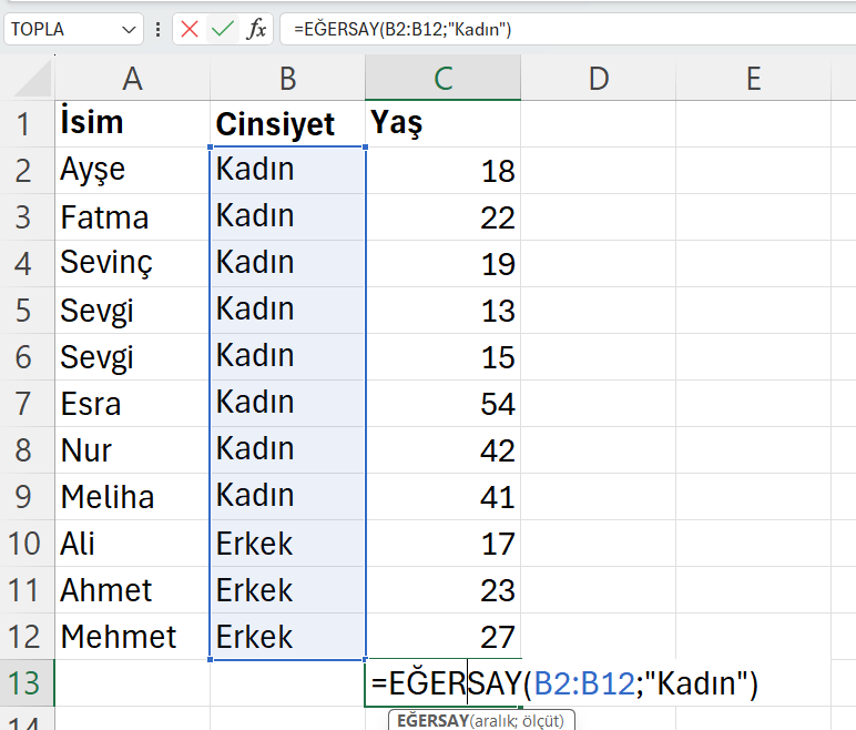
=COUNTIF(B2:B12;“Female”) Finds How Many of the Searched Value Exist. Finds How Many Cells Contain “Female” from B2 to B12.
You can use ornek2a.xlsx file for the following examples
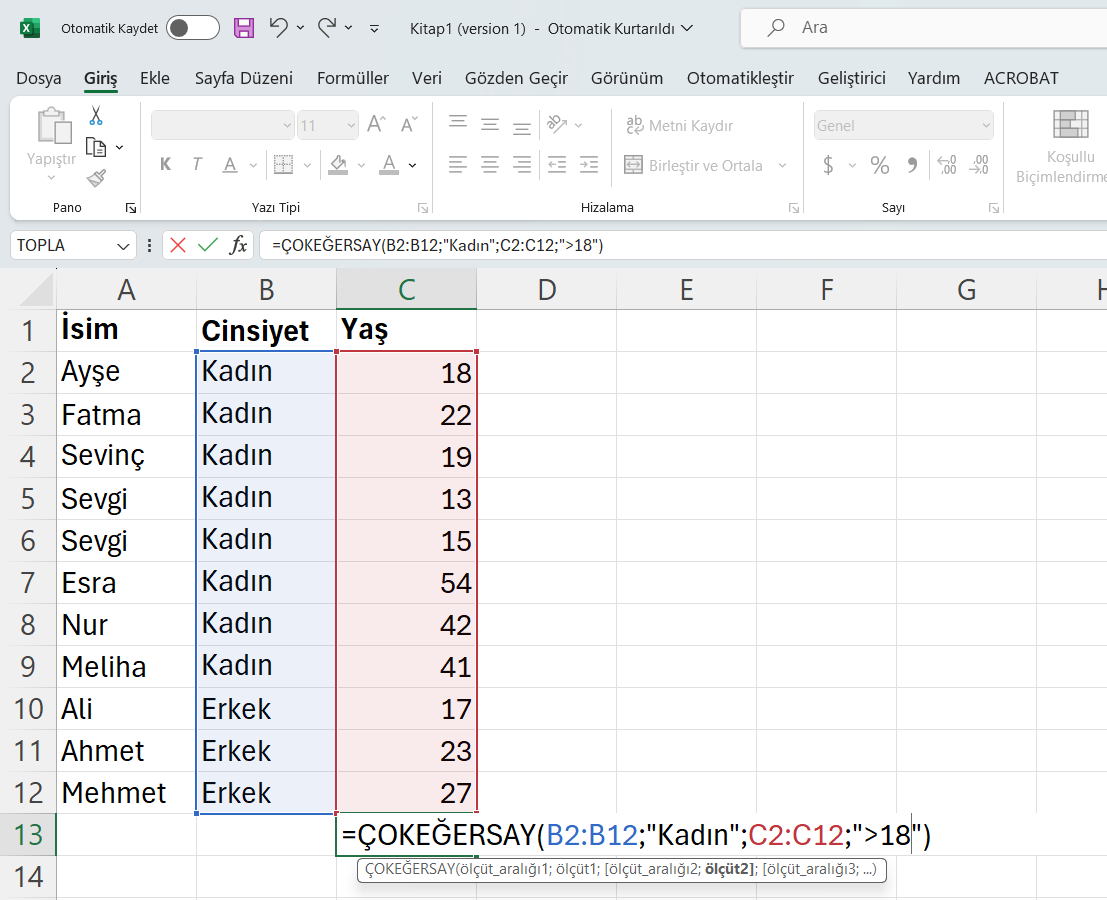
COUNTIFS(B2:B12;“Female”;C2:C12;“>18”) Finds How Many Match Multiple Search Criteria. Finds How Many Cells Contain “Female” Value from B2 to B12 AND Are Greater Than 18 from C2 to C12.
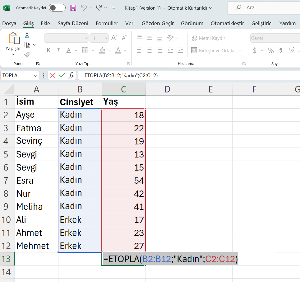
=SUMIF(B2:B12;“Female”;C2:C12) Finds the Sum of the Range That Matches the Search Value. Finds the Sum of the Range from C2 to C12 Corresponding to Cells Containing “Female” from B2 to B12.
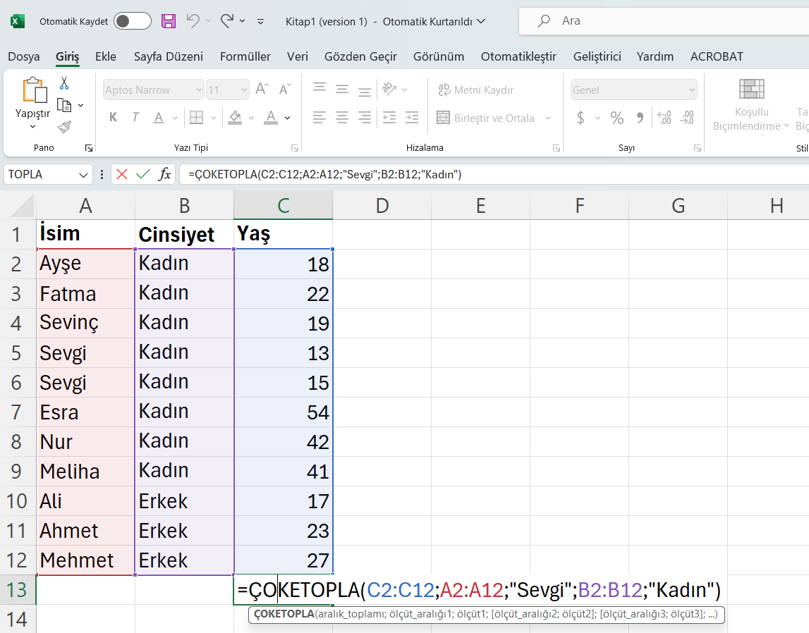
=SUMIFS(C2:C12;A2:A12;“Sevgi”;B2:B12;“Female”) Finds the Sum of the Range That Matches Multiple Search Values. This formula sums the ages of those named Sevgi and who are Female.
=AVERAGEIF(B2:B12;“Female”;C2:C12) Calculates the Average of Values Corresponding to Cells That Match the Search Criteria. Finds “Female” Values from B2 to B12 And Calculates the Average of Their Corresponding Values from C2 to C12.
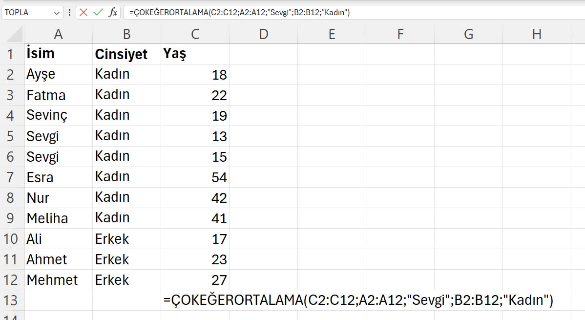
=AVERAGEIFS(C2:C12;A2:A12;“Sevgi”;B2:B12;“Female”) Calculates the Average of Values Corresponding to Cells That Match Multiple Search Criteria. Finds “Female” Values. Finds “Sevgi” Values. Takes Average of Ages.
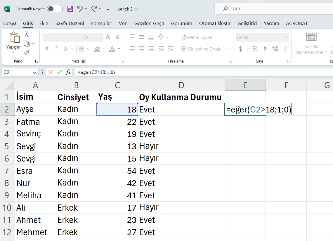
IF Function
This function allows for evaluating outcomes based on whether a condition is met or not.
Usage format: =IF(condition;true result;false result)
condition can be written by comparing a cell with a number or comparing values of two cells.
true result is the expression or value to be written when the condition is met.
false result is the expression or value to be written when the condition is not met.
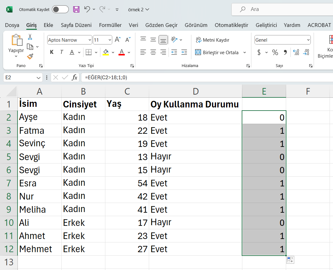
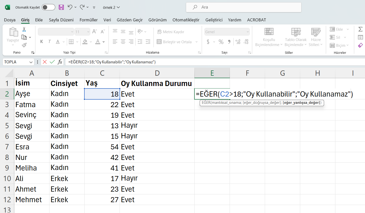
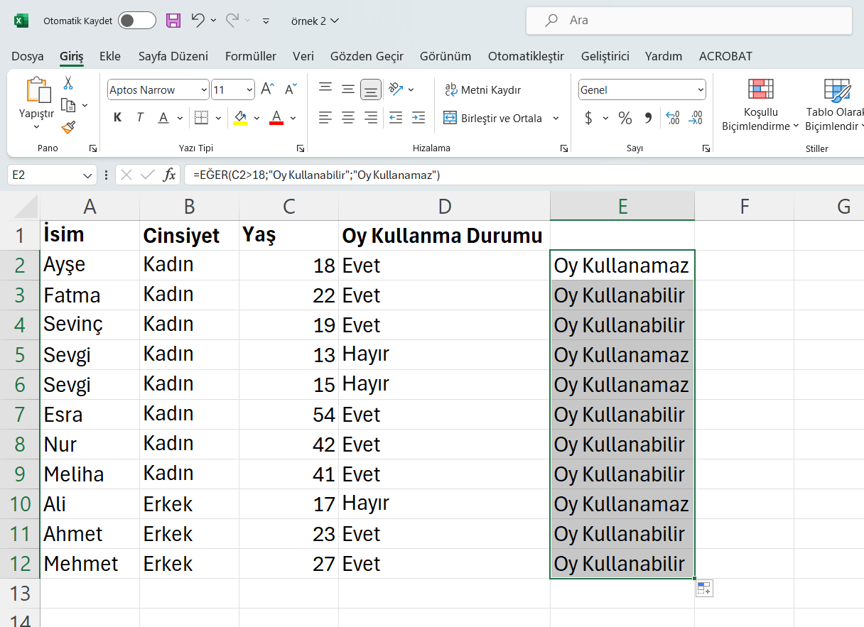
Let’s Look at the Examples Below.
We assigned label 1 to True Result and 0 to False Result. After writing the first function, we can copy the same function for other cells by dragging the cells.
We assigned “Can Vote” to True Result and “Cannot Vote” to False Result. After writing the first function, we can copy the same function for other cells by dragging the cells.
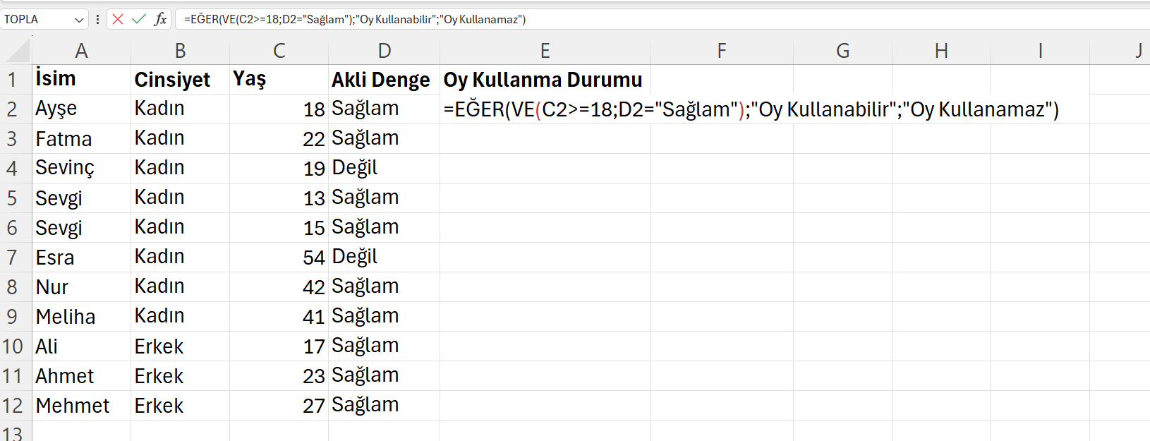
AND and OR Operators
When you need to check multiple conditions in an IF function, you can use AND operator or OR operator. If you want all multiple conditions to be met for a positive result in the IF function, use the AND operator; if meeting just one of the conditions is sufficient, write the formula with the OR operator.
Let’s add another column to the above table (Mental Status)
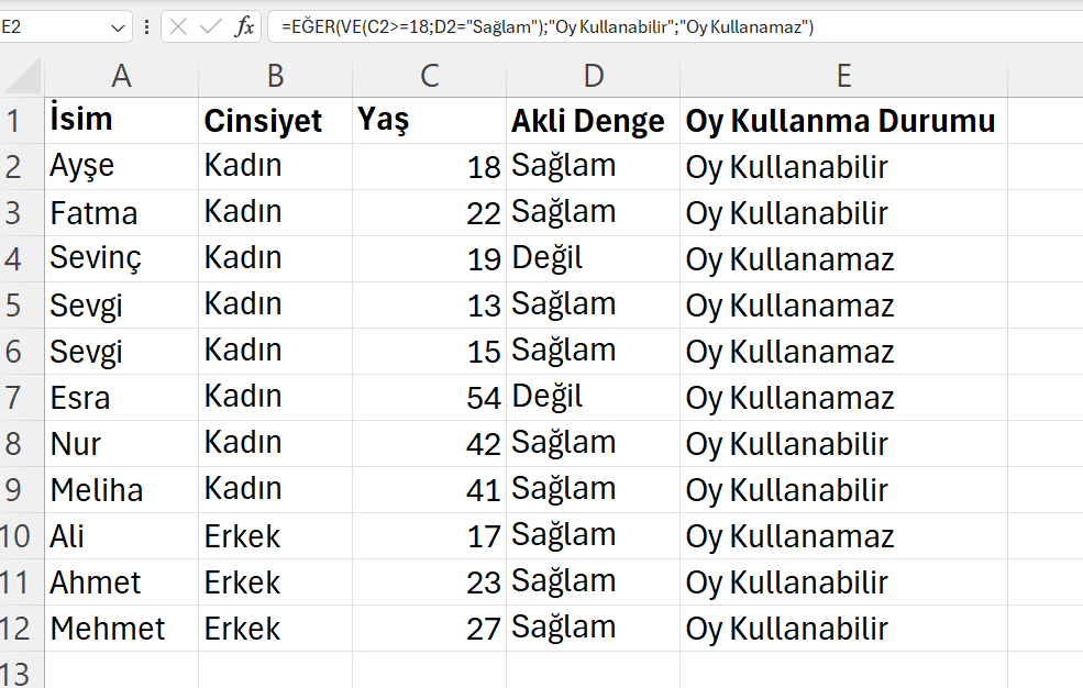
If age is 18 and mental status is sound, they can vote. That is, both conditions must be met.
You can use file ornek2b.xlsx for the following examples
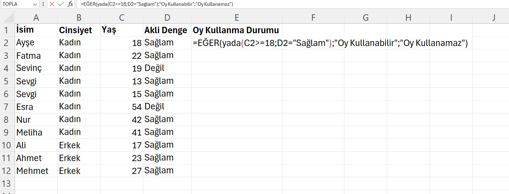
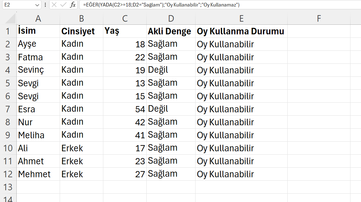
If age is 18 or mental status is sound, they can vote. Meeting one condition is sufficient.
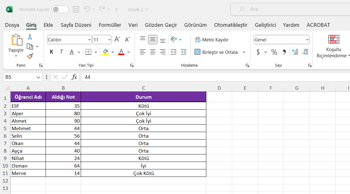
Nested IF
Let’s say we have students and their grades. We want to show students who got:
- 80 - 100 as “Very Good”
- 60 - 79 as “Good”
- 40 - 59 as “Average”
- 20 - 39 as “Poor”
- 0 - 19 as “Very Poor”
Let’s examine the following function:
=IF(B2>=80;“Very Good”;IF(B2>=60;“Good”;IF(B2>=40;“Average”;IF(B2>=20;“Poor”;“Very Poor”))))
You can use file ornek3.xlsx for the following examples